Rambling On Randomness
What is randomness
According to the Oxford Dictionary, “the randomness is the apparent lack of pattern or predictability in events”. Randomness implies “Unpredictability”. To practically illustrated it: if a sequence of numbers is given and you have no way to predict what the next number in the sequence will be - then the sequence is random. A single number cannot ever be random. 13…ok…not random. But: 1, 3, 5, 7, 9, 11, 13 …the ‘13’ doesn’t seem very random because you could have predicted it with almost complete certainty.
Theoretical Approach
Central Limit Theorem
Mathematically, if $X_{1}, X_{2}, \ldots, X_{n}$ is a random sample of size $n$ taken from a population with mean $\mu$ and finite variance $\sigma^{2}$ and if $\bar{X}$ is the sample mean, the limiting form of the distribution of $Z=\left(\frac{X-\mu}{\sigma / N / N}\right)$ as $n \rightarrow \infty$, is the standard normal distribution. There are no constraints on the distribution of the input signal. It can be anything, even if the distribution of the source signal does not seem like the Gaussian Distribution, eventually, the sample means will be converged to Gaussian Distribution.
Berry-Essen Theorem
In probability theory, the central limit theorem states that, under certain circumstances, the probability distribution of the scaled mean of a random sample converges to a normal distribution as the sample size increases to infinity. Under stronger assumptions, the Berry–Esseen theorem, or Berry–Esseen inequality, gives a more quantitative result, because it also specifies the rate at which this convergence takes place by giving a bound on the maximal error of approximation between the normal distribution and the true distribution of the scaled sample mean.
$$\left|F_{n}(x)-\Phi(x)\right| \leq \frac{C \rho}{\sigma^{3} \sqrt{n}}$$
Where: C is a constant, Fn is the cumulative distribution function, and $\theta$ is the cumulative distribution function of the standard normal distribution.
Gödel’s Incompleteness Theorems
It is not possible at all to say is a finite series of numbers is random or not. It is a consequence of the Gödel’s incompleteness theorems 1. For example, if there is a number generators which creates numbers from 1 to 10 and it is creating the sequence of “2 2 2 2 2 2 2 2”. However it still can be the part of a random series and you just saw a lucky (unlucky) sequence. On the other hand “4,9,1,5,5,7,2,1,1,9,5,6” is not also indicates randomness. Our source could following a certain sequence and it start to repeat after $(n+1)^{th}$ step.
Practical Examples
Statistical Analysis
The histograms of the random sequence can give information about whether the sequence is random or not. Histogram show the discrete distribution the samples. Therefore, according to sample distribution it is possible to make predictions about the randomness of the signal.
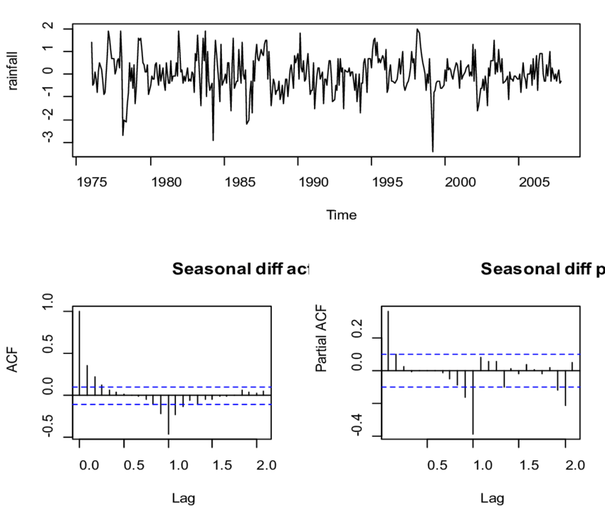
The second method can be the auto-correlation test. Auto-correlation is a method to calculate the self similarity and repeated patterns of the sequence. For this purpose, the sequence is lagged and correlation coefficient is calculated with the lagged version of itself.
Compressibility
One of the property which indicates the randomness is compressibility. Kolmogorov randomness states that is a signal is not random it should be compressible 2. Furthermore there is a theory depends on this fact which is “Compressed Sensing”. According to this theory, the natural signals should be compressible. Therefore, for example their total variation should be small. Using this theory, Total variation is used as constraint during the optimization to keep the total variation of the signal smaller. Therefore noisy signals are cleaned with this method.
True Random Generators
The true random generator is investigated since it should provide a high amount of randomness. It is a piece of hardware equipment that creates truly random samples when it is needed. Randomness is used in lots of places in computers such as video rendering, cryptography, and programming. Therefore, these devices are developed to feed computer programs with random numbers. When these devices are designed, the pseudo-randomness is generated with high entropy input sources 3. The generated sample at t, should not give any information about the sample before the t or the sample after the t.
Conclusion
In the end, according to the probability theory, true randomness can not be proven. For engineering purposes, it is only defined according to requirements and can be measured to detect non-randomness or patterns. This may bring the question “Is the true randomness exist?”. Maybe one-day physics can answer that question certainly. According to the latest theories, Quantum physics suggests that truly random events occur on the basis of Heisenberg’s Uncertainty Principle.