mozanunal.com / Posts / Human Activity Recognition with LSTM Networks
Human Activity Recognition with LSTM Networks
· 10 min read
Table of Contents
Hello everyone! In this post, I will recognize what a person is doing, such as walking, sitting, or climbing stairs, from the accelerometer and gyroscope of a smartphone. I will compare four models: a classic neural network on hand crafted features, a plain LSTM, a CNN LSTM, and a Convolutional LSTM, trained on the UCI Smartphone dataset and on a small dataset I recorded myself.
Results in short: the plain LSTM reached 90.6% validation accuracy, the CNN LSTM 91.8%, and the Convolutional LSTM 89.1%, while the feature based baseline stayed around 78%. The CNN LSTM was both the most accurate and much faster to train than the plain LSTM.
Human Activity Recognition
Human activity recognition (HAR) is a popular machine learning problem, and recent work shows that deep networks, especially LSTMs, do very well on it [1]. Almost every phone and smartwatch carries the two sensors that matter most:
- Accelerometer: measures linear acceleration along three axes, typically within a range of a few g.
- Gyroscope: measures angular velocity around three axes.
The two complement each other. The accelerometer is noisy while the device is moving, and the gyroscope drifts over time, so their readings are usually combined with sensor fusion to get a reliable estimate of the device’s motion and orientation.
A typical HAR pipeline looks like the figure below. Sensor data is collected, often sent to the cloud, cleaned and filtered, and then passed to a deep learning model that extracts features and classifies the activity. Deep learning makes it possible to recognize more complex activities, and the more complex the activities we can recognize, the more useful HAR becomes. As the number of wearables grows, so does the amount of data and the compute needed to process it, which is why accurate and cost effective models matter.
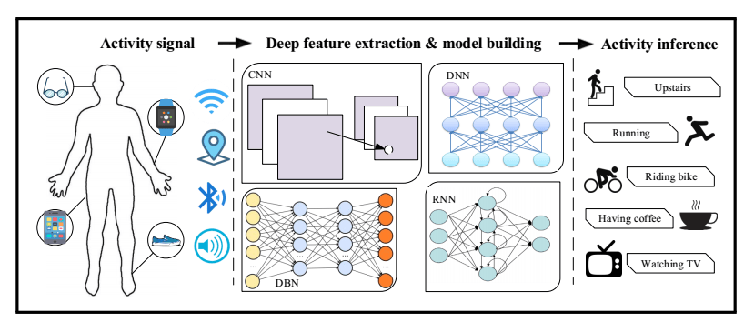 Human activity recognition pipeline
Datasets
UCI Smartphone Dataset
The UCI HAR dataset [2] was recorded from 30 volunteers aged 19 to 48, each wearing a smartphone on the waist while performing six activities: walking, walking upstairs, walking downstairs, sitting, standing, and lying down. Each session was video recorded and labelled by hand. Sensors were sampled at 50 Hz and the signals are split into windows of 128 samples (2.56 seconds).
After preprocessing, the training set has 7352 windows and the validation set has 2947. Each window is 128 time steps long with 9 channels (body and total acceleration plus angular velocity, each on three axes), and each label is a one hot vector over the 6 classes.
My Own Dataset
I also collected a small dataset with a phone app I wrote in DroidScript. It has 80 recordings from 4 people sampled at 20 Hz, with labels that describe the context as well as the movement: sitting in a car, at home, on a bus, at a computer, or on the metro, standing on a bus or on the metro, standing while waiting, walking outside, and running. After splitting into windows of 100 samples (5 seconds), there are 708 training and 178 validation windows, each with 7 channels.
The label distributions are shown below. The UCI dataset is well balanced, while mine is not, since some activities were simply much easier to record for longer.
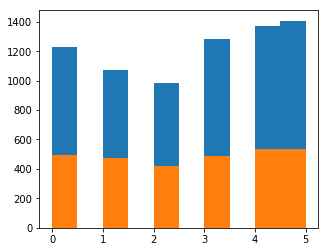
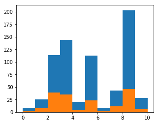 Label distribution of the UCI dataset (top) and my own dataset (bottom)
Preprocessing
For the deep models, I did not compute any hand crafted features and fed the raw signals directly. The data was normalized per person, so that differences between how individuals move or carry their phone matter less, then split into windows and shuffled. The network never sees which person a window came from.
Models
Baseline: Hand Crafted Features and a Dense Network
As a baseline, each window is summarized with a set of classic features per axis: the maximum, the standard deviation, the skewness, and frequency domain values. This turns every window into a 396 dimensional feature vector, which is classified by a small fully connected network.
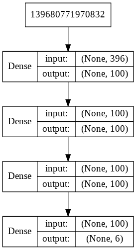 Layers of the feature based baseline network
LSTM
Recurrent neural networks (RNNs) give a network memory by feeding the output of a step back into the next step. You can picture them as the same cell unrolled over the sequence.
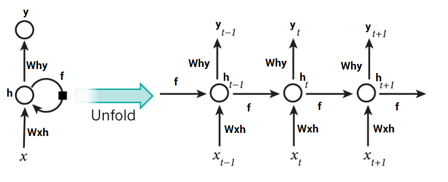 An RNN unrolled over time [3]
Plain RNNs struggle with long sequences, which is known as the problem of long-term dependencies. The hidden state passes through a nonlinearity at every step, and the gradients that flow back through all these steps tend to vanish or explode. In practice, information from early in the sequence gets lost.
The LSTM solves this with a second path through the cell, the cell state, often called the conveyor belt. It is the top line in the figure below, and it is only touched by an elementwise multiplication (the forget gate) and an addition (the input gate). With no squashing nonlinearity on this path, information and gradients can survive across many more time steps [3].
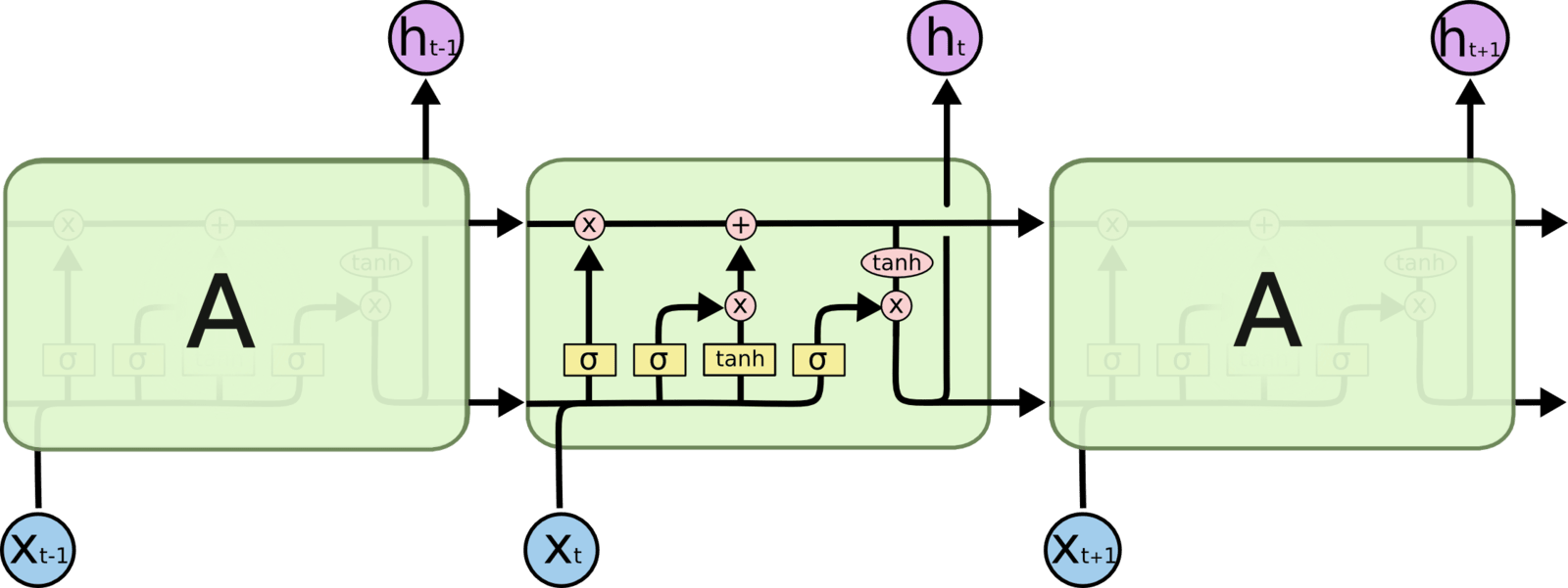 Structure of an LSTM cell [3]
The LSTM model I used has four layers. It takes a 128 x 9 window and outputs a probability for each of the 6 classes.
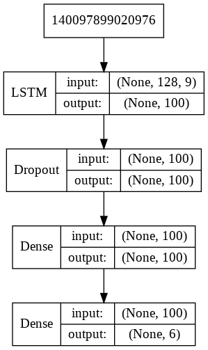 Layers of the LSTM model
CNN LSTM
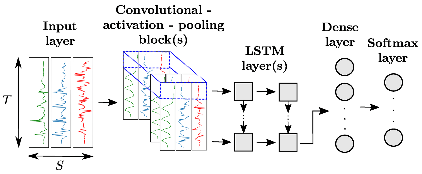
The CNN LSTM works in two stages [4]. First, 1D convolutions extract local features from short chunks of the window. These features are flattened and passed as a much shorter sequence to the LSTM layers, which model how they change over time and make the final prediction.
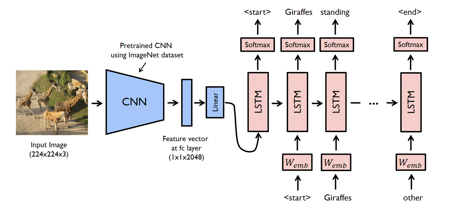 Structure of a CNN LSTM network
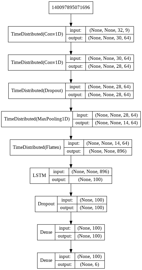 Layers of the CNN LSTM model
Convolutional LSTM
The Convolutional LSTM (ConvLSTM) [5] goes one step further and puts the convolution inside the LSTM cell itself: the input to state and state to state transitions are convolutions instead of matrix multiplications. The signal is treated as a 2D array, like an image, and unlike the CNN LSTM the outputs are not flattened before the recurrent part.
 Structure of a Convolutional LSTM network
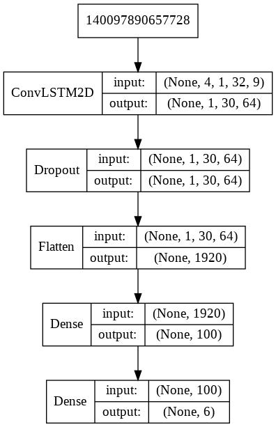 Layers of the Convolutional LSTM model
Loss Function and Training
All four models end with a fully connected softmax layer that outputs class probabilities. They are trained with the categorical cross entropy loss:
$$CE = -\sum_{i=1}^{C} t_i \log(s_i)$$
where $C$ is the number of classes, $t_i$ is 1 for the correct class and 0 otherwise, and $s_i$ is the predicted probability of class $i$. The loss is small when the model puts a high probability on the correct class.
Training minimizes this loss with the Adam optimizer, a variant of gradient descent. Each step runs a forward pass to compute the loss, uses backpropagation to compute the gradient of the loss with respect to every weight, and moves the weights a small step against the gradient. This repeats for every batch, over many epochs.
Results
All models were trained on an NVIDIA K80 GPU in Google Colab. For each model, the first pair of plots shows accuracy and loss on the training and validation sets per epoch, and the second pair shows confusion matrices for the training and validation sets.
Baseline
The feature based network trains in about a second per epoch, but it overfits heavily: training accuracy goes up to 99% while validation accuracy stays around 78%.
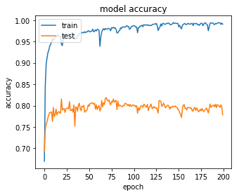
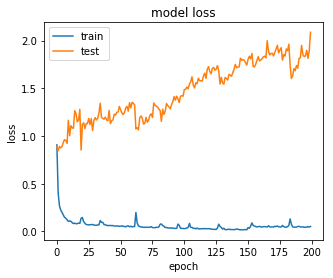 Final epoch: loss 0.052, accuracy 99.1%, validation loss 2.087, validation
accuracy 77.8%
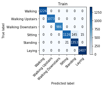
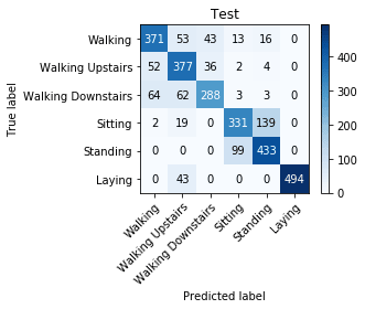 Confusion matrices for the baseline network
LSTM
The LSTM ran for 60 epochs at about 42 seconds each. The loss went down for almost the whole run, apart from a sudden spike around epochs 13 to 16. It ended at 90.6% validation accuracy.
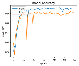
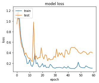 Final epoch: loss 0.105, accuracy 95.6%, validation loss 0.398, validation
accuracy 90.6%
The confusion matrices show where the errors come from: sitting and standing. Both are static postures, and with a phone on the waist they produce very similar signals, so the LSTM cannot reliably tell them apart. On the validation set, about 200 sitting and standing windows are swapped. The walking classes have a few mix ups, and lying down is classified perfectly.
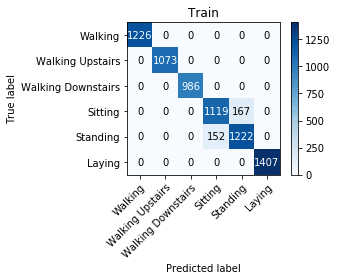
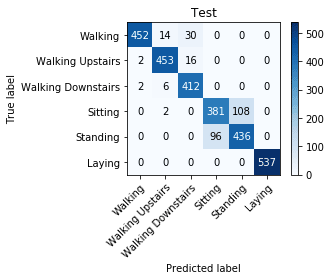 Confusion matrices for the LSTM
CNN LSTM
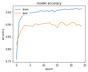
The CNN LSTM is the most complex architecture here, yet it trains much faster: about 17 seconds per epoch, and 25 epochs were enough. The convolutions shrink the 128 step window into a much shorter sequence of features, so the LSTM has far fewer sequential steps to process, and convolutions themselves parallelize well on a GPU. It reached the best validation accuracy, 91.8%.
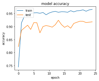
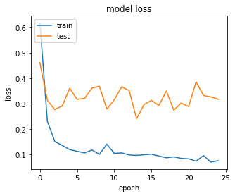 Final epoch: loss 0.076, accuracy 96.6%, validation loss 0.318, validation
accuracy 91.8%
Sitting and standing remain the main source of confusion. The gain over the plain LSTM is mostly in training time rather than accuracy.
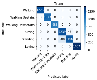
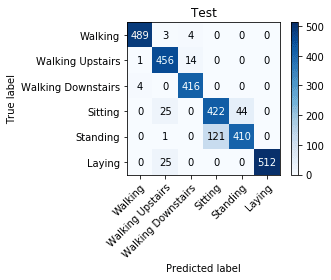 Confusion matrices for the CNN LSTM
Convolutional LSTM
The Convolutional LSTM learns fastest: it passes 90% validation accuracy after only 5 epochs, at about 29 seconds each, which makes it attractive for larger datasets. However, its validation loss is noticeably higher, and it finished at 89.1% validation accuracy.
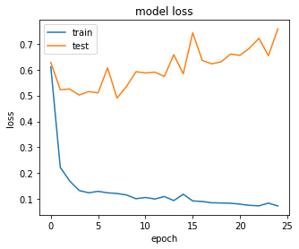 Final epoch: loss 0.074, accuracy 96.5%, validation loss 0.757, validation
accuracy 89.1%
It separates sitting and standing slightly better than the plain LSTM, but in exchange it confuses the walking classes more, often predicting walking downstairs for walking or walking upstairs. It also labels some sitting and lying down windows as walking upstairs, which the other models never do.
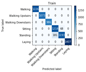
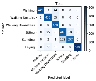 Confusion matrices for the Convolutional LSTM
LSTM on My Own Dataset
Finally, I trained the LSTM on my own dataset. With far less data, an epoch took only 2 seconds, and after 60 epochs the validation accuracy was 90.4%.
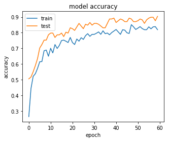
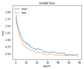 Final epoch: loss 0.461, accuracy 81.9%, validation loss 0.375, validation
accuracy 90.4%
The biggest confusion is between standing on a bus and standing while waiting. Both are mostly standing still with small movements, so this is not surprising.
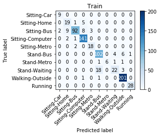
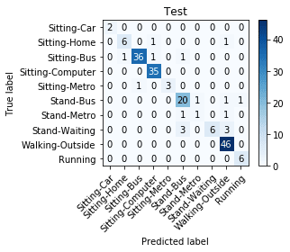 Confusion matrices for the LSTM on my own dataset
Summary
| Model | Validation accuracy | Time per epoch | Epochs |
|---|---|---|---|
| Features + dense network | 77.8% | about 1 s | |
| LSTM | 90.6% | 42 s | 60 |
| CNN LSTM | 91.8% | 17 s | 25 |
| Convolutional LSTM | 89.1% | 29 s | 5 to reach 90% |
| LSTM, own dataset | 90.4% | 2 s | 60 |
Conclusion
LSTMs work very well on long sensor time series and give solid results without much compute or any hand crafted features. Putting convolutional feature extractors in front of the LSTM, as in the CNN LSTM, gave the best accuracy and cut training time by more than half, since the LSTM only has to process a compact sequence of features. The remaining errors come mostly from activities that look the same to a waist mounted sensor, such as sitting and standing.
Future Work
- Test the models on the UCSD ExtraSensory dataset, which captures behavioral context in the wild from phones and smartwatches [6].
- Try feature extraction, signal filtering, other normalization schemes, and data augmentation on that dataset to improve accuracy.
- Apply the same models to accelerometer based gesture recognition, for example the SmartWatch Gestures dataset [7].
References
- T. Zebin, N. Peek, A. Casson, and M. Sperrin, “Human activity recognition from inertial sensor time-series using batch normalized deep LSTM recurrent networks,” in Proc. IEEE EMBC, 2018.
- D. Anguita, A. Ghio, L. Oneto, X. Parra, and J. L. Reyes-Ortiz, “Human Activity Recognition on Smartphones Using a Multiclass Hardware-Friendly Support Vector Machine,” in Ambient Assisted Living and Home Care, Springer, 2012.
- C. Olah, “Understanding LSTM Networks,” 2015. https://colah.github.io/posts/2015-08-Understanding-LSTMs/
- T. N. Sainath, O. Vinyals, A. Senior, and H. Sak, “Convolutional, Long Short-Term Memory, fully connected Deep Neural Networks,” in Proc. IEEE ICASSP, 2015.
- X. Shi, Z. Chen, H. Wang, D.-Y. Yeung, W.-K. Wong, and W.-C. Woo, “Convolutional LSTM Network: A Machine Learning Approach for Precipitation Nowcasting,” arXiv:1506.04214, 2015.
- Y. Vaizman, K. Ellis, and G. Lanckriet, “Recognizing Detailed Human Context in the Wild from Smartphones and Smartwatches,” IEEE Pervasive Computing, vol. 16, no. 4, 2017.
- L. Porzi, S. Messelodi, C. Modena, and E. Ricci, “A smart watch-based gesture recognition system for assisting people with visual impairments,” 2013.
← Electrical Impedance Tomography: How It Works and Where It Is Used | Yolo on Google Colab →